Chi Square Test Vs Fisher Exact Updated
Chi Square Test Vs Fisher Exact
What are contingency tables?
Contingency tables provide the integer counts for measurements with respect to 2 categorical variables. The simplest contingency table is a \(ii \times two\) frequency table, which results from two variables with two levels each:
| Group/Observation | Observation 1 | Observation 2 |
|---|---|---|
| Grouping i | \(n_{1,1}\) | \(n_{1,ii}\) |
| Group 2 | \(n_{2,1}\) | \(n_{2,ii}\) |
Given such a table, the question would be whether Group 1 exhibits frequencies with respect to the observations than Group ii. The groups represents the dependent variable because they depend on the observation of the contained variable. Note that it is a common misconception that contingency tables must be \(2 \times 2\); they can have an capricious number of dimensions, depending on the number of levels exhibited by the variables. Still, performing statistical tests on contingency tables with many dimensions should be avoided because, amidst other reasons, interpreting the results would be challenging.
The warpbreaks information set
To study tests on contingency tables, we volition use the warpbreaks data prepare:
information(warpbreaks) caput(warpbreaks) ## breaks wool tension ## one 26 A 50 ## two thirty A 50 ## three 54 A L ## 4 25 A L ## 5 lxx A L ## 6 52 A L This is a information set with 3 variables originating from the textile manufacture: breaks describes the number of times there was a break in a warp thread, \(\text{wool} \in \{A, B\}\) describes the type of wool that was tested, and \(\text{tension} \in \{Fifty, M, H\}\) gives the tension that was applied to the thread (either low, medium, or high). Each row in the data gear up indicates the measurements for a single loom. To account for the variability of dissimilar looms, 9 measurements were performed for each combination of wool and tension, the data gear up contains a full of \(9 \cdot 2 \cdot 3 = 54\) observations.
Goal of the analysis
Nosotros would similar to identify whether 1 type of wool outperforms the other for different levels of tensions. To investigate whether we tin find some prove for differences, permit'south have a expect at the data:
To investigate the differences in the number of strand breaks, permit'south visualize the data:
library(ggplot2) ggplot(warpbreaks, aes(x = tension, y = breaks)) + facet_wrap(. ~ wool) + geom_boxplot() 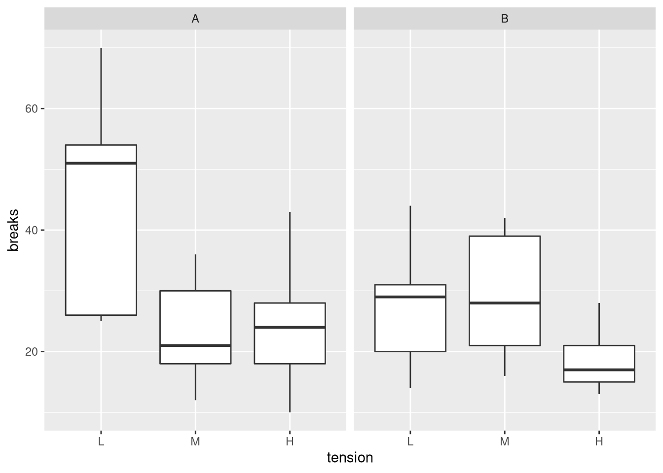
From the plot, we can meet that, overall, wool B is associated with fewer breaks. Wool A seems to be particularly inferior for low tensions.
Transformation to contingency table
To obtain a contingency table, we first need to summarize the breaks beyond unlike looms for the two types of wool and the three types of tension.
library(plyr) df <- ddply(warpbreaks, .(wool,tension), summarize, breaks = sum(breaks)) impress(df) ## wool tension breaks ## 1 A L 401 ## ii A Grand 216 ## 3 A H 221 ## iv B L 254 ## 5 B Grand 259 ## vi B H 169 We then utilise the xtabs (pronounced as crosstabs) part to generate the contingency table:
df <- xtabs(breaks~wool+tension, data = df) print(df) ## tension ## wool 50 M H ## A 401 216 221 ## B 254 259 169 Now, df has the structure we need for applying statistical tests.
Statistical testing
The ii well-nigh common tests for determining whether measurements from different groups are independent are the chi-squared examination (\(\chi^ii\) exam) and Fisher'south exact test. Note that you should use McNemar's exam if the measurements were paired (eastward.g. individual looms could be identified).
Pearson's chi-squared examination
The \(\chi^2\) exam is a non-parametric exam that tin can be practical to contingency tables with various dimensions. The proper noun of the exam originates from the \(\chi^two\) distribution, which is the distribution for the squares of independent standard normal variables. This is the distribution of the test statistic of the \(\chi^2\) test, which is defined by the sum of chi-square values \(\chi_{i,j}^2\) for all pairs of cells \(i,j\) arising from the difference between a cell'south observed value \(O_{i,j}\) and the expected value \(E_{i,j}\), normalized by \(E_{i,j}\):
\[\sum \chi_{i,j}^two \quad \text{where} \quad \chi_{i,j}^2 = \frac{(O_{i,j}−E_{i,j})^2}{E_{i,j}}\]
The intuition here is that \(\sum \chi_{i,j}^2\) will be big if the observed values considerably deviate from the expected values, while \(\sum \chi_{i,j}^two\) will exist close to zero if the observed values concord well with the expected values. Performing the examination via
chi.result <- chisq.test(df) print(chi.outcome$p.value) ## [1] 7.900708e-07 Since the p-value is less than 0.05, we can pass up the null hypothesis of the test (the frequency of breaks is independent of the wool) at the 5% significance level. Based on the entries of df one could then claim that wool B is significantly improve (with respect to warp breaks) than wool A.
Investigating the Pearson residuals
Some other fashion would exist to consider the chi-foursquare values of the test. The chisq.examination function, provides the Pearson residuals (roots) of the chi-square values, that is, \(\chi_{i,j}\). In dissimilarity to the chi-foursquare values, which result from squared differences, the residuals are not squared. Thus, residuals reflect the extent to which an observed value exceeded the expected value (positive value) or cruel short of the expected value (negative value). In our data set, positive values indicate more strand breaks than expected, while negative values betoken less breaks:
print(chi.consequence$residuals) ## tension ## wool 50 M H ## A 2.0990516 -ii.8348433 0.4082867 ## B -2.3267672 3.1423813 -0.4525797 The residuals bear witness that, compared with wool A, wool B had less breaks for low and high tensions than expected. For, medium tension, nevertheless, wool B had more breaks than expected. Once again, nosotros find that, overall wool B is superior to wool A. The values of the residuals also bespeak that wool B performs best for depression tensions (rest of 2.1), well for high tensions (0.41) and badly for medium tensions (-2.8). The residuals, all the same, helped us in identifying a problem with wool B: it does not perform well for medium tension. How would this inform further development? In order to obtain a wool that performs well for all tension levels, we would demand to focus on improving wool B for medium tension. For this purpose, nosotros could consider the properties that make wool A perform better at medium tension.
Fisher's exact examination
Fisher's verbal test is a non-parametric exam for testing independence that is typically used only for \(2 \times two\) contingency tabular array. As an exact significance test, Fisher's exam meets all the assumptions on which basis the distribution of the test statistic is defined. In practice, this means that the fake rejection rate equals the significance level of the examination, which is not necessarily true for approximate tests such as the \(\chi^two\) test. In short, Fisher's verbal test relies on computing the p-value co-ordinate to the hypergeometric distribution using binomial coefficients, namely via
\[p = \frac{\binom{n_{1,one} + n_{ane,ii}}{n_{1,1}} \binom{n_{2,1} + n_{2,2}}{n_{2,i}}}{\binom{n_{ane,1} + n_{1,ii} + n_{two,1} + n_{ii,2}}{n_{1,i} + n_{two,1}}}\]
Since the computed factorials can become very large, Fisher'due south verbal exam may not piece of work for large sample sizes.
Note that it is non possible to specify the alternative of the test for df since the odds ratio, which indicates the effect size, is only divers for \(two \times two\) matrices:
\[OR = {\frac{n_{1,one}}{n_{1,two}}}/{\frac{n_{2,ane}}{n_{2,2}}}\]
We tin can still perform Fisher'southward exact test to obtain a p-value:
fisher.event <- fisher.test(df) impress(fisher.result$p.value) ## [i] 8.162421e-07 The resulting p-value is like to the one obtained from the \(\chi^2\) test and we go far at the same conclusion: we can reject the null hypothesis that the type of wool is independent of the number of breaks observed for different levels of stress.
Conversion to 2 past 2 matrices
To specify the alternative hypothesis and obtain the odds ratio, nosotros could compute the examination for the three \(2 \times 2\) matrices that tin be constructed from df:
p.values <- rep(NA, 3) for (i in seq(ncol(df))) { # compute strand breaks for tested stress vs other types of stress test.df <- cbind(df[, i], apply(df[,-i], 1, sum)) tested.stress <- colnames(df)[i] colnames(test.df) <- c(tested.stress, "other") # for clarity test.res <- fisher.test(test.df, alternative = "greater") p.values[i] <- test.res$p.value names(p.values)[i] <- paste0(tested.stress, " vs others") } Since the alternative is set to greater, this means that we are performing a one-tailed test where the alternative hypothesis is that wool A is associated with a greater number of breaks than wool B (i.e. we expect \(OR > i\)). Past performing tests on \(2 \times ii\) tables, we also gain interpretability: we tin can now distinguish the specific weather under which the wools are different. Earlier interpreting the p-values, yet, we need to correct for multiple hypothesis testing. In this case, we have performed three tests. Here, nosotros'll simply adjust the initial significance level of 0.05 to \(\frac{0.05}{3} = 0.01\overline{6}\) co-ordinate to the Bonferroni method. Based on the adjusted threshold, the following tests were meaning:
impress(names(p.values)[which(p.values < 0.05/3)]) ## [one] "L vs others" This finding indicates that wool B is merely significantly superior to wool A if the stress is light. Note that we could accept too the approach of amalgam \(2 \times 2\) matrices for the \(\chi^two\) test. With the \(\chi^2\) exam, even so, this wasn't necessary because we based our analysis on residuals.
Summary: chi-squared vs Fisher's exact test
Here is a summary of the properties of the two tests:
| Benchmark | Chi-squared exam | Fisher's verbal test |
|---|---|---|
| Minimal sample size | Large | Small |
| Accuracy | Approximate | Verbal |
| Contingency table | Capricious dimension | Usually 2x2 |
| Interpretation | Pearson residuals | Odds ratio |
By and large, Fisher'southward exact exam is preferable to the chi-squared test because it is an exact test. The chi-squared test should exist particularly avoided if there are few observations (e.m. less than ten) for individual cells. Since Fisher's exact examination may exist computationally infeasible for big sample sizes and the accurateness of the \(\chi^2\) examination increases with larger number of samples, the \(\chi^2\) test is a suitable replacement in this case. Another advantage of the \(\chi^ii\) exam is that it is more suitable for contingency tables whose dimensionality exceeds \(2 \times 2\).

Lamentable
Your mail service has non been submitted. Please render to the form and brand sure that all fields are entered. Thank You!
Chi Square Test Vs Fisher Exact
Posted by: garciadrandrus00.blogspot.com
0 Response to "Chi Square Test Vs Fisher Exact Updated"
Post a Comment